Since the 1990s, satellite missions have provided a wealth of SAR imagery for Earth monitoring applications. However, due to the complex nature of SAR images and the limited availability of labeled datasets, these images remain underutilized as reference information for machine learning. To address this gap, we designed a SAR feature creation workflow within an operational framework and made the related Jupyter tools publicly available.
The workflow, built upon Doris-5, consists of four main components (Figure 1).
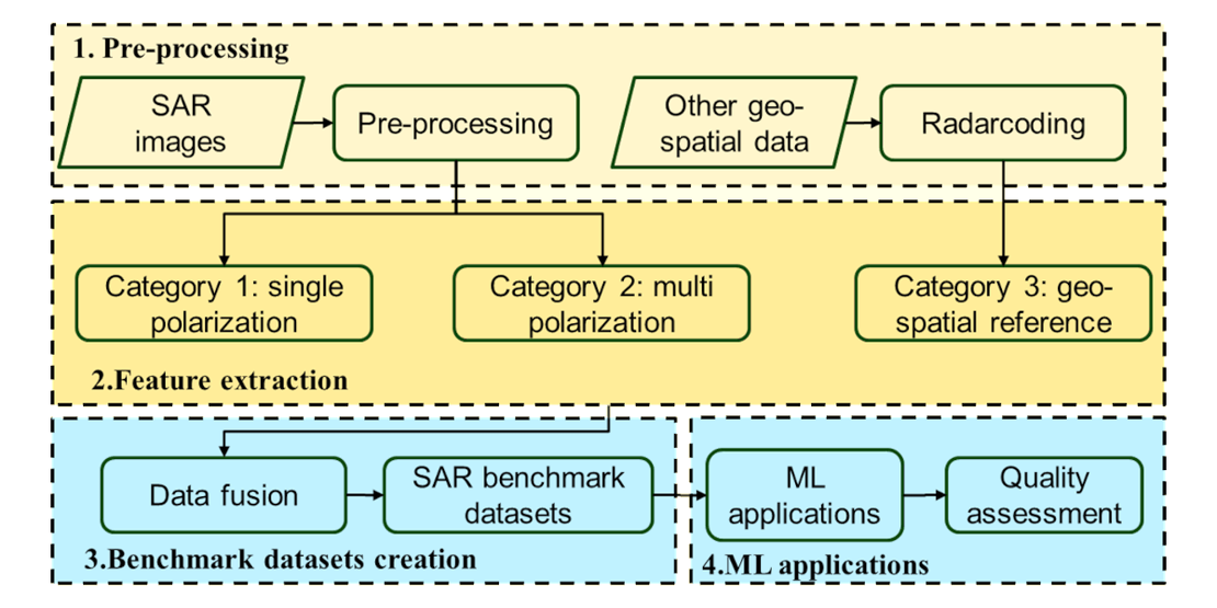
Figure 1. Proposed workflow with pre-processing, feature extraction, benchmark datasets creation, and ML application blocks.
The first component involves the pre-processing of SAR images and the transformation of available geospatial datasets, such as optical imagery, cadastral maps, and geological maps, to generate additional features for SAR data that can serve as reference information. The pre-processed SAR images and radar-coded reference data are extracted according to three categories, and aligned as feature images in the second block. In the third block, the quality of feature images is assessed, and images are fused into standard SAR benchmark datasets. These benchmark datasets are then applied and tested in the fourth block using various machine learning methods. All SAR features are concatenated as separate layers in the NetCDF data format, which incorporates Spatio-Temporal Asset Catalogs (STAC) to support efficient data querying.
For demonstration purposes, an area in the province of Groningen, The Netherlands, was selected as the test site. Seven ascending Sentinel-1A images in VV and VH modes on track 15, captured between January and March 2022, were used along with the TOP10NL topographic dataset as a reference (Figure 2).
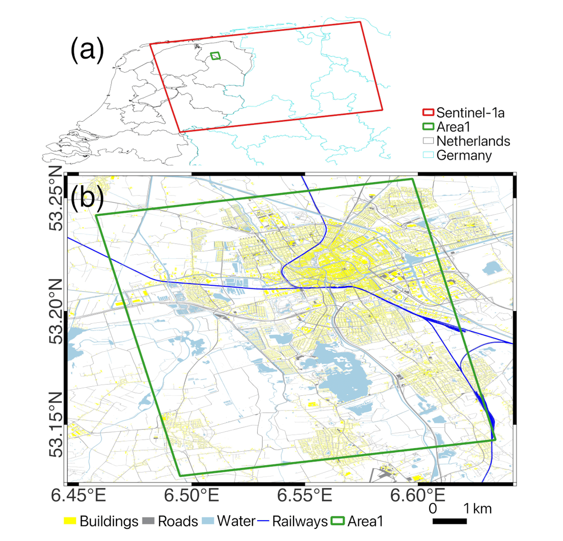
Figure 2. The study area in Groningen, The Netherlands. (a) shows the coverage of the Sentinel-1 image, with the AOI, in green, partly covering the city of Groningen, (b) is the zoomed-in of the green AOI in (a), describing Groningen city with the LULC classes of buildings, roads, water, and railways.
The extracted features included VV amplitude, VH amplitude, VV interferometric phase, VV coherence, intensity summation, intensity difference, intensity ratio, cross-polarization correlation coefficient, cross-polarization cross product, and entropy. Additionally, features representing buildings, roads, water bodies, and railways were extracted. The first ten features were generated according to Categories 1 and 2, while the latter four were produced following Category 3 specifications (Figure 3).
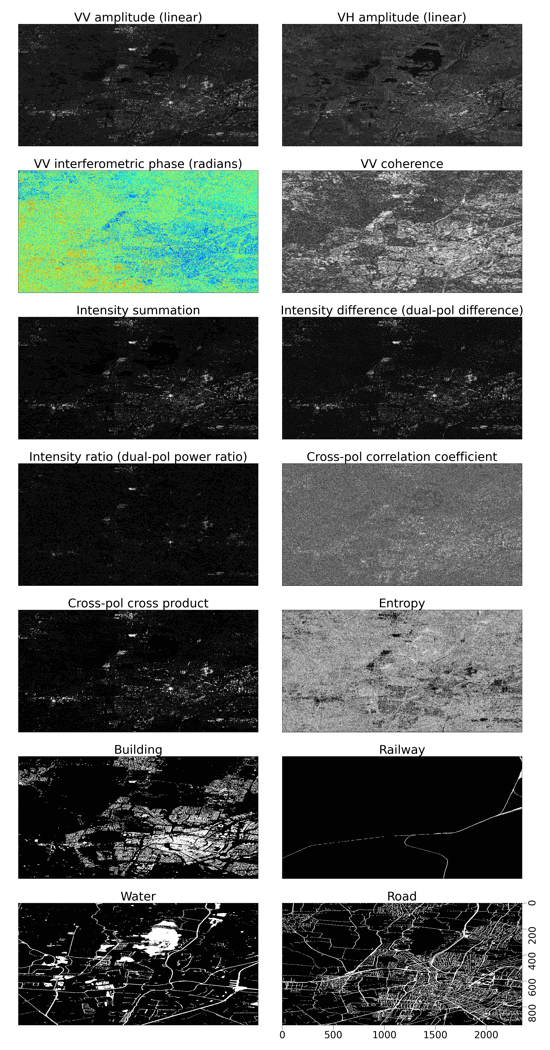
Figure 3. 14 SAR features for the acquisition on 9 January 2022 in Groningen.
By applying a random forest classifier to these fourteen SAR features, the model produced four types of classified SAR images: building, road, water, and railway. The overall accuracy for the acquisition on 9 January 2022 was 0.8558, 0.9939, 0.9065, and 0.8191, respectively, with corresponding F1-scores of 0.9191, 0.9669, 0.9490, and 0.9006. As the number of training samples increased in subsequent acquisitions, the model demonstrated improved predictive performance across different classes (Figure 4).
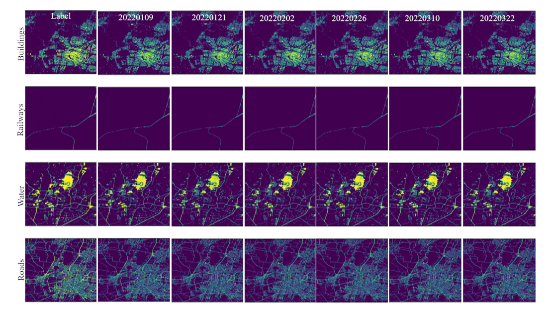
Figure 4. Four landcover types in rows including buildings, railways, water, and roads. The first column is label while the rest are predicted results of corresponding dates.
One of the primary challenges we faced was storage requirements. SAR images are inherently large (each raw image is around 4 GB) and the processing steps produced substantial intermediate outputs, collectively reaching several hundred gigabytes. Additionally, pre-processing and transforming the reference dataset, TOP10NL, into radar coordinates demanded significant computational power. Compounding these challenges, the processing tool DORIS 5 required a Linux environment and relied on outdated dependencies such as Python 2, which caused compatibility issues with modern software packages. Fortunately, access to the Geospatial Computing Platform (GCP) enabled us to effectively address these technical and infrastructural hurdles.
The GCP serves as a robust computing infrastructure, offering extensive storage capacity and seamless compatibility across Linux systems, including support for older software packages in isolated environments. It also accommodates diverse computational needs by integrating Jupyter Notebook for interactive analysis while enabling the use of multiple programming languages. The CRIB team provided invaluable support throughout the process, assisting with software and package installation. Their prompt responses, insightful discussions, and proactive monitoring of hardware and algorithm performance made the research process not only productive but also highly encouraging and enjoyable.
For more information about the study please contact to Xu Zhang.