In this exercise, a simple slope stability model (the infinite slope model) is used to calculate safety factor maps for different conditions. The effect of groundwater depth and seismic acceleration is evaluated using input maps of these factors for different return periods of rainfall (related to the groundwater level) and earthquakes (related to the seismic acceleration).
In ILWIS, the model is represented by a user-defined function. Different scenarios are calculated by changing the variables of this function. The model is applied on a data set of the city of Manizales, in central Colombia.

Introduction and data preparation

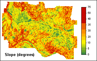
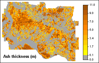
Two of the input maps are a slope map and a map of ash thickness:

The degree of slope hazard can be expressed by the Safety Factor (F) which is the ratio of the forces that make a slope fail and those that prevent a slope from failing.

• F < 1 unstable slope conditions,
• F = 1 slope is at the point of failure,
• F > 1 stable slope conditions.

To simplify matters, the infinite slope model is used. This is a 2-dimensional model describing the stability of slopes with an infinitively large failure plane.

The depth of the possible failure plane is taken at the contact of the volcanic ashes and the underlying material. The consequence of that is that safety factors will not be calculated for the entire area, but only for the areas where there is volcanic ash at the surface.

The formula to calculate the Safety Factor (Brunsden and Prior, 1979) reads:

With some Mapcalc calculations in which you will use the inbuilt ILWIS functions DEGRAD( ), SIN( ), COS( ), and SQ( ), first some maps are prepared that will be frequently used in this application:

• map SI, sine of slope
• map CO, cosine of slope
• map CO2, squared cosine of slope

Creating a user-defined function for the infinite slope model, and calculating Safety Factors for various groundwater scenarios

The Safety Factor formula as presented above will be transformed into a user-defined function FS. This function already contains the known parameters (maps ASHT, SI, CO, CO2 and the known constants) but it also contains the variables Gamma and m.

The function can then be easily applied for various heights of the watertable (z_w), by filling out the variables Gamma and m. This will result in a number of Safety Factor maps for specific watertable heights.

Function FS reads:
(10000+((Gamma-m*10000)*ASHT*CO2*0.58)) / (Gamma*ASHT*SI*CO)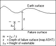

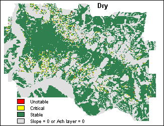
• For the dry scenario, Gamma = 11000, and without water z_w=0 and thus m=0 as well.
  To obtain a map with Safety Factors for the dry scenario (FSDRY), function FS is applied using parameters 11000 and 0.
  FDRY = FS(11000,0)
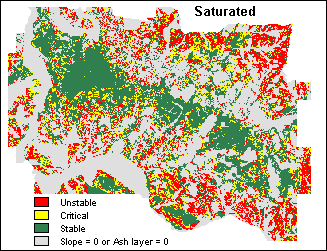
• For the saturated scenario, Gamma = 16000, and when all soil above the failure surface is saturated with water, z_w=z thus m=1.
  A map with Safety Factors for the saturated scenario (FSAT) is then calculated by using function FS with parameters 16000 and 1.
  FSAT = FS(16000,1)

The maps are (re)classified according to:

Subsequently, function FS is applied repeatedly on the command line and Safety Factor maps are calculated for a number of watertable height scenarios. For each scenario, a value for Gamma is provided and the values for m are found in a number of existing groundwater maps (M016, M1, M20, M50).

Safety Factors are calculated for groundwater peaks that occur:

during two months a year (rather dry):	Gamma=14000, m=M016
once a year:	Gamma=14000, m=M1
once in every 20 years:	Gamma=14000, m=M20
once in every 50 years (very wet):	Gamma=14000, m=M50
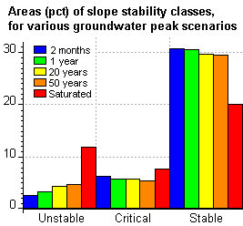Of all maps, histograms are calculated and the area percentages of the stability classes are joined into one table. From the table, a bar graph is presented. The graph displays the relative size of the areas that are found to be unstable, critical and unstable slopes for different groundwater level scenarios.

Evaluating the effect of seismic acceleration

Besides groundwater fluctuations, also earthquake acceleration will be taken into account.
The formula for the infinite slope model changes into:

Compared to the original formula (see above), the new parameters are:

z_w can be replaced with m*z, as m=z_w/z.
This formula thus contains the known parameters (maps ASHT, SI, CO, CO2 and the known constants) but it also contains the variables gamma, m, rho and alpha.

Another user-defined function has to be created (FSNEW), which may read:

(10000+(ASHT*Gamma*CO2-ASHT*Rho*Alpha*CO*SI-10000*m*ASHT*CO2)*0.58) / (ASHT*Gamma*SI*CO+ASHT*Rho*Alpha*CO2)

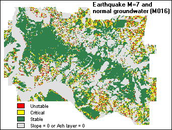
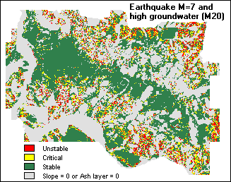
With user-defined function FSNEW and some additional information, Safety Factors are then calculated for the following scenarios:

1. Dry condition, without earthquake.
2. Ground water return period of 20 years, without earthquake.
3. Completely saturated situation, without earthquake.
4. Dry condition, and earthquake of 7 Magnitude.
5. Groundwater with return period of 0.16 years, and earthquake of 7 Magnitude.
6. Groundwater with return period of 20 years, and earthquake of 7 Magnitude.

In order to compare the output maps, all maps are (re)classified according to:

Results of scenarios 5 and 6 are displayed below:

For more information on this case study, contact:

C.J. van Westen
Department of Earth Systems Analysis,
International Institute for Geo-Information Science and Earth Observation (ITC),
P.O. Box 6, 7500 AA Enschede, The Netherlands.
Tel: +31 53 4874263, Fax: +31 53 4874336, e-mail: westen@itc.nl