ILWISPy Getting Started

Getting started with ILWISPy, Python and Jupyter notebooks

Ben Maathuis, Bas Retsios, Martin Schouwenburg, Willem Nieuwenhuis and Lichun Wang.
Faculty ITC, University of Twente. March 2022.

Why ILWISPy

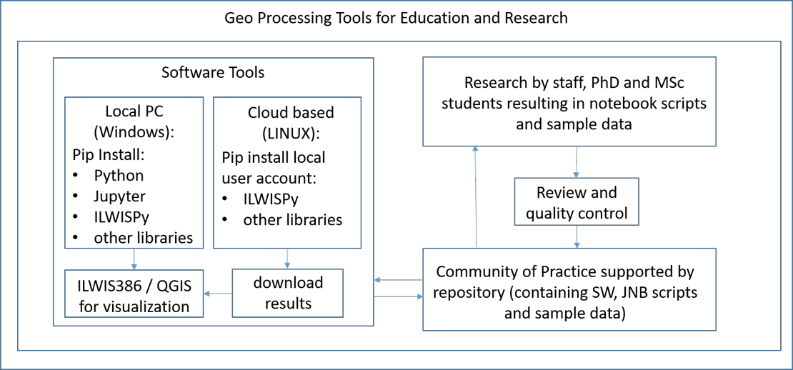
ILWISPy is a Geo‐Processing Tool which can be used as a site‐package under Python. The main objective of ILWISPy is to 'achieve more with less coding' and 'increase flexibility'. ILWISPy has a large library of commonly used GIS and RS operations which can be easily coded through single line statements. The core is based on C++ and is fast. This capability, together with other Python sitepackages, offers great flexibility in data retrieval, (pre‐) processing and analysis, far exceeding those offered through Graphical User Interface (GUI) Geo‐processing tools.

ILWISPy can be directly imported in Python, but can also be used within a Jupyter Notebook, offering the capability of markdown text with explanations and subsequent coding fields to execute certain operations, which for educational purposes offers nice opportunities. For research applications these notebooks and data used contribute to ‘open science’ showing all processing steps conducted.

For quick display of results or more advanced visualizations use can be made of exiting free GUI based software tools like ILWIS386 or QGIS.

Figure 1: Role of ILWISPy in education and research.

Disclaimer

At the moment of writing this document the following limitations should be noted:

ILWISPy is currently available as a Python wheel for:

• Python36 and higher as Windows 64 bits
• Python38 for LINUX Ubuntu

This document describes installation on a Windows OS system from scratch, without previous installation of Python, Conda or mini-Conda. If (mini-) Conda has been installed already then another installation procedure should be followed. Additional information can be obtained from the authors. 

Temporary issue related to the use of ILWISPy under Jupyter Notebook. After installation of the Jupyter Notebook site package and subsequent installation of ILWISPy, within your Python folder:

• rename file 'Python_folder'\DLLs\sqlite3.dll to 'Python_folder'\DLLs\sqlite3_dll.orig
• copy the file sqlite3.dll from 'Python_folder'\Lib\site-packages\ILWIS\ilwisobjects\extensions\gdalconnector\ to 'Python_folder'\DLLs\

All resources, including Python and some wheels, are also available at:
https://filetransfer.itc.nl/pub/52n/ilwis_py/. The following structure is adhered to:

• /notebooks: Notebooks in Jupyter Notebook format and as HTML. The JNB format files can be directly used, just copy and paste these in your local notebook folder. The HTML files show the full processed content of the notebook, to show the user what is to be expected and output created by execution of the notebook
• /sample_data: data used within the notebooks
• /wheels: the ILWISPy wheels, for Windows and Linux‐Ubuntu. User can select the required wheel version according to their local Python version used. 
• /temporary_tools: additional resources, including the python36 installer, shortcut and icon for Jupyter notebook as well as a number of wheels that are used on a frequent basis. 

1.1. install Python for Windows

Visit the Python download pages at: https://www.python.org/downloads/.

As example for preparation of this document Python version 3.6 is used, but same instructions are applicable when using a higher Python versions. Select under "Looking for a specific release?" Python Release version "Python 3.6.8" (https://www.python.org/downloads/release/python-368/) and download the ‘Windows x86-64 executable installer’.

To install Python on your system (assumed here a Windows – 64 bits operating system):

1. Double click with the mouse the file "python‐3.6.8‐amd64.exe", activate the option "Add Python 3.6 to PATH" and select the installation option "Customize installation";
2. In the next window "Optional Features" continue with "Next";
3. Use the default settings in the "Advanced Options" window, but change under the "Customize Install Location" the folder settings to: "C:\Python36".
4. Press “Install” and accept the system request to make changes to your configuration;
5. After installation Python will indicate if the installation was successful and press "Close".

Navigate with your system "Explorer" to the newly created folder "C:\Python36" and click on the icon in front of the folder settings (see Figure 2), this should now receive a blue color, subsequently type, using the keyboard "CMD", to open the command line interpreter in the folder "C:\Python36".

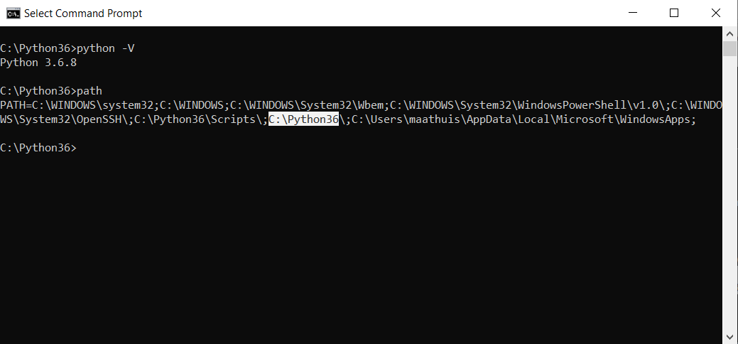
Type the following syntax: "python --version" or "python -V" and you should get the information about the version installed. Next type "path", to check if the path is set to the python folder, here: "c:\python36", see Figure 3.

Figure 2: Python 3.6 folder content showing the executable "python.exe".

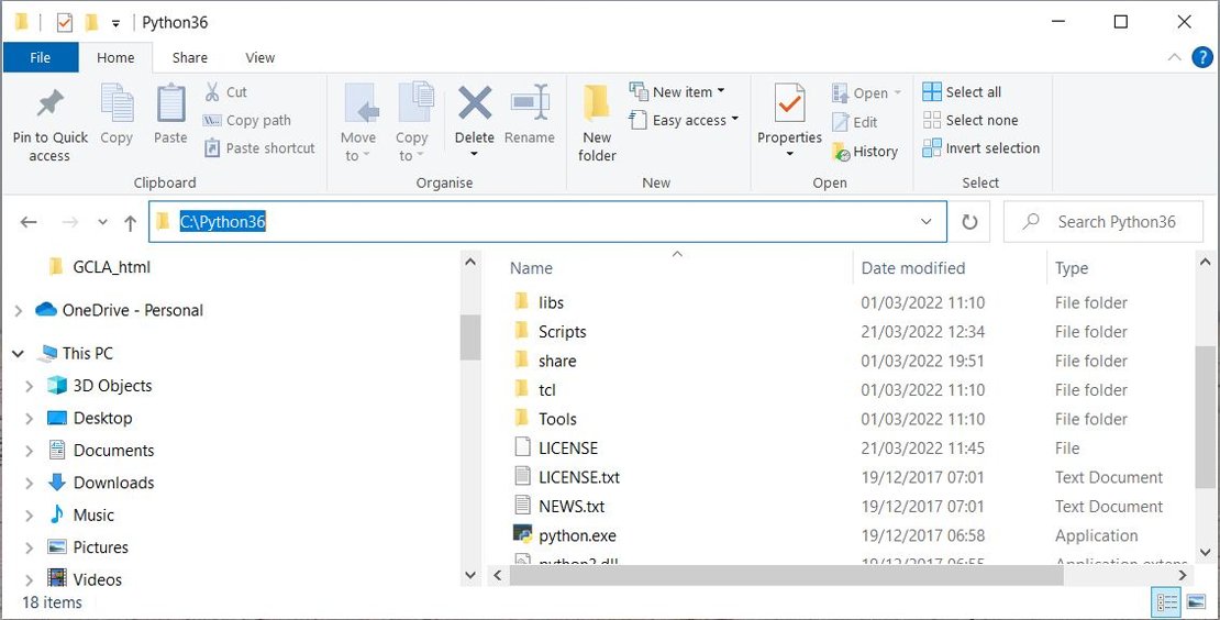
Figure 3: Check Python version installed and your system path settings.

1.2 Install ILWISPy

Navigate to the folder https://filetransfer.itc.nl/pub/52n/ilwis_py/wheels/windows/ and download the wheel file, for example: 'ilwis-1.0-cp36-cp36m-win_amd64.whl'. Select the wheel according to the local python version used. After download, copy this file to a local folder on your system.

Open again the command prompt window, see figure 2, and ensure that you are in the python36 folder. From the command prompt, type the following command:

Note: replace 'drive\local folder' with the location of your actual drive:\folder on your system.

Once ILWISPy is installed you will get a message "Successfully installed ilwis‐Version_number"

To check the installation, type the following expressions on the command prompt:

To close Python press <Ctrl>Z and press <Enter> or type: exit()

Note that ILWISPy is installed under the Python36 folder, in \Lib\site‐packages\ilwis. You can check the content, also check the folder \Lib\site‐packages\ilwis‐Version_number.dist‐info. The file ‘Metadata’ can be opened using Notepad, providing additional information on the version used and point of contact and other resources.

To uninstall ILWISPy:

1.3 Install Python libraries

Python makes use of some libraries which have to be installed separately. A library is a collection of pre‐combined codes that can be used iteratively to reduce the time required to code. They are particularly useful for accessing the pre‐written frequently used codes, instead of writing them from scratch every single time. Similar to the physical libraries, these are a collection of reusable resources, which means every library has a root source. This is the foundation behind the numerous open‐source libraries available in Python.

Pip is a useful program to install additional libraries in Python. To ensure you are working with the latest version of pip, type the following command from within the python36 folder:

Mind: there are 2 dashes without space -- before the upgrade command above.

To install additional libraries use the following command from within the python folder:

Some useful libraries for data science are:

• NumPy: Numerical Python is the fundamental package for numerical computation in Python; it contains a powerful N‐dimensional array object.
• Matplotlib: Matplotlib is a plotting library for Python. Because of the graphs and plots that it produces, it’s extensively used for data visualization.
• SciPy: Scientific Python is another free and open‐source Python library for data science that is extensively used for high‐level computations.
• Pandas: Python data analysis is a must in the data science life cycle. It is the most popular and widely used Python library for data science, along with NumPy in Matplotlib.

Install the libraries mentioned above, replacing “some library” with the names mentioned above, like numpy, matplotlib, etc. If additional libraries are going to be used at a later stage, you will be asked to install them before you continue.

A number of additional libraries, in case required, are available (as whl) at: 
https://filetransfer.itc.nl/pub/52n/ilwis_py/temporary_tools/.
Note that installation of these wheels is the same as for ILWISPy, using: python ‐m pip install *.whl

Now with Python, ILWISPy and the required libraries installed we continue with the installation of the Jupyter notebook.

1.4 Install Jupyter Notebook

Installing Jupyter notebook under Python using pip install:

• The command to install Jupyter is similar as given above: “python ‐m pip install jupyter”.
  Type this command in the cmd window in the folder “c:\python36”; 
• First a number of files are downloaded and then the Packages are installed;
• Once finished the installation create a new folder on the root of your c:\drive, e.g. “Jupyter” and navigate to this folder in an identical manner as shown in Figure 1, but now using the folder ”c:\jupyter”;
• From the folder “c:\jupyter” type the following command to launch Jupyter notebook using command‐line: “jupyter notebook”. Your default browser is opened, e.g. “Chrome” and you can navigate to the respective JNB files or sub‐folders were your notebooks are residing;
• If you want to use ILWISPy under Jupyter Notebook, see last bullet under ‘Disclaimer’.

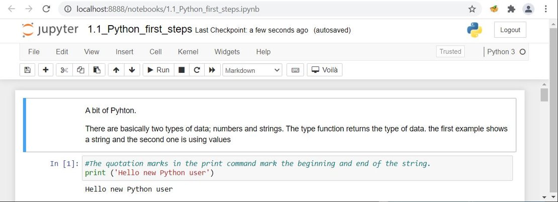
Navigate to: https://filetransfer.itc.nl/pub/52n/ilwis_py/notebooks/As_JNB/python_intro/. Copy the sample notebooks, e.g. “1.1_Python_fist_steps.ipynb” to “1.9_Python_fist_steps.ipynb to the folder “C:\jupyter”.

Click on the notebook “1.1_Python_fist_steps.ipynb” to get started. You should get the content as of Figure 4.

Figure 4: Starting the Jupyter notebook using the first lesson.

1.5 Create shortcut

From https://filetransfer.itc.nl/pub/52n/ilwis_py/temporary_tools/ copy the files “Jupyter.lnk” (shortcut) and “jnb_ico” to the folder c:\jupyter. Ensure that the extension of the file Jupyter.lnk remains the same (could be renamed to download!)

Within your folder c:\jupyter,drag the shortcut “Jupyter.lnk” to the desktop. Right click the shortcut, inspect the properties, ensure that the “Start in” folder is correct, here: c:\jupyter. Also click the button “Change Icon” and navigate to the folder c:\jupyter\ and select the file “jnb.ico”.

Double click the shortcut to start a ‘Jupyter Notebook’ session. If you have installed the notebooks in a different folder, right click the shortcut with the mouse and change the properties accordingly, e.g. the properties under “Start in”. Now close all active windows.

1.6 Intro to Jupyter Notebook

A notebook integrates code and its output into a single document that combines visualizations, narrative text, mathematical equations, and other rich media. In other words: it's a single document where you can run code, display the output, and also add explanations, formulas, charts, and make your work more transparent, understandable, repeatable, and shareable.

Jupyter’s Notebooks and dashboard are web apps, and Jupyter starts up a local Python server to serve these apps to your web browser, making it essentially platform‐independent and opening the door to easier sharing your code developed on the web.

Start Jupyter NoteBook (JNB) by double clicking the shortcut created and open once more the notebook ”1.1_Python_fist_steps.ipynb”. The dashboard’s interface is mostly self‐explanatory. Each .ipynb file is a text file that describes the contents of your notebook in a format called JSON. Each cell and its contents, including image attachments that have been converted into strings of text, is listed therein along with some metadata.

There are two items appearing in the main menu that you should notice: cells and kernels. These are key both to understanding Jupyter and to what makes it more than just a word processor.

A kernel is a “computational engine” that executes the code contained in a notebook document. A cell is a container for text to be displayed in the notebook or code to be executed by the notebook’s kernel. Cells form the body of a notebook. There are two main cell types:

• A Code cell contains code to be executed in the kernel. When the code is run, the notebook displays the output below the code cell that generated it.
• A Markdown cell contains text formatted using Markdown and displays its output in‐place when the Markdown cell is run.

You can always tell the difference between Code and Markdown cells because code cells have that label on the left and Markdown cells do not. The “In” part of the label is simply short for “Input,” while the label number indicates when the cell was executed on the kernel. In a Jupyter Notebook, there is always one “active” cell highlighted with a border whose color denotes its current mode:

• Green outline — cell is in "edit mode"
• Blue outline — cell is in "command mode"

To run a cell press the Shift + Enter keys simultaneously. There are plenty of other commands we can use. The best way to use them is with keyboard shortcuts. Keyboard shortcuts are a very popular aspect of the Jupyter environment because they facilitate a speedy cell‐based workflow. Many of these are actions you can carry out on the active cell when it’s in command mode.

Below, you’ll find a list of some of Jupyter’s keyboard shortcuts. You don't need to memorize them all immediately, but this list should give you a good idea of what’s possible.

• Toggle between edit and command mode with Esc and Enter, respectively.
• Once in command mode:
  • Scroll up and down your cells with your Up and Down keys.
  • Press ‘a’ or ‘b’ to insert a new cell above or below the active cell.
  • ‘m’ will transform the active cell to a Markdown cell.
  • ‘y’ will set the active cell to a code cell.
  • ‘d’ + ‘d’ (d twice) will delete the active cell.
  • ‘z’ will undo cell deletion.
  • Hold Shift and press Up or Down to select multiple cells at once. With multiple cells selected, Shift + ‘m’ will merge your selection.
• Ctrl + Shift + ‐, in edit mode, will split the active cell at the cursor. If your keyboard has more than one key corresponding to ‐, and one zooms out instead of splitting cells, try using the other key. 
• You can also click and Shift + Click in the margin to the left of your cells to select them.

From the “Help” menu also additional information about the various keyboard shortcuts can be obtained.

Markdown is a lightweight, easy to learn markup language for formatting plain text. Markdown is a lightweight and popular Markup language which is a writing standard for data scientists and analysts. It is often converted into the corresponding HTML by the Markdown processor which allows it to be easily shared between different devices and people.

Markup language is similar to Hypertext Markup Language (HTML) made of Markup tags, and it consists of the opening tag <tagname> and closing tag </tagname>. For additional information on Markdown, see: https://www.datacamp.com/community/tutorials/markdown‐in‐jupyter‐notebook.

Behind every notebook runs a kernel. When you run a code cell, that code is executed within the kernel. Any output is returned back to the cell to be displayed. The kernel’s state persists over time and between cells — it pertains to the document as a whole and not individual cells.

For example, if you import libraries or declare variables in one cell, they will be available in another.

Most of the time when you create a notebook, the flow will be top‐to‐bottom. But it’s common to go back to make changes. When we do need to make changes to an earlier cell, the order of execution we can see on the left of each cell, such as ‘In [6]’ (in front of a cell), can help diagnose problems by seeing what order the cells have run in.

And if we ever wish to reset things, there are several useful options from the Kernel menu:

• Restart: restarts the kernel, thus clearing all the variables etc. that were defined.
• Restart & Clear Output: same as above but will also wipe the output displayed below your code cells.
• Restart & Run All: same as above but will also run all your cells in order from first to last.
• If your kernel is ever stuck on a computation and you wish to stop it, you can choose the Interrupt option.

Depending on the type of installation, Jupyter provides the option to change the kernel – programming languages. Many other languages, in addition to Python, may be used in the notebook. By creating a new notebook from the dashboard menu, by selecting Python, you are actually choosing which kernel to use. Here only the Python kernel is at your disposal.

Open the command line interpreter in the folder “C:\Python36”, see figure 2. Type the following syntax: “jupyter kernelspec list” and you should get the information about the kernel installed, here ‘python3’.

1.7 Jupyter Notebooks samples

From: https://filetransfer.itc.nl/pub/52n/ilwis_py/notebooks/As_JNB/python_intro/:

A sequence of sample notebooks on Intro Python – scripting are prepared to guide you through the different aspects of using python and subsequent processing capability offered. The notebook filenames are numbered, e.g. 1.1_* to 1.9_*, covering some of the required python background.

Go through the notebooks in this sequential order, once a notebook is opened use the Shift+Enter keys to go through the fields in the notebook and execute the sample code given.

From https://filetransfer.itc.nl/pub/52n/ilwis_py/notebooks/As_HTML/:

The Notebooks are now saved as HTML, these show you the results of the code fields executed, so you can compare your results obtained by execution of the notebook with those shown in the HTML version.

1.8 References and resources

Allen Downey (2015): Think Python. How to Think Like a Computer Scientist. 2nd Edition, Version 2.4.0. Green Tea Press. Available at: https://greenteapress.com/thinkpython2/thinkpython2.pdf

Attard, Guillaume (2021): An Intro to the Earth Engine Python API. Available at:
https://developers.google.com/earth-engine/tutorials/community/intro-to-python-api

Khan, S. (2020): Learn Basic Statistics with Python. Available at:
https://medium.com/insights-school/learn-basic-statistics-with-python-cc0f45275929

Sat Kumar Tomer (2011): Python in Hydrology. Green Tea Press. Available at:
https://www.greenteapress.com/pythonhydro/pythonhydro.pdf

Stojiljkovic, M. Python Statistics Fundamentals: How to Describe Your Data. Available at:
https://realpython.com/python-statistics/

Qiusheng Wu. Earth Engine Py Notebooks. A collection of 360+ Jupyter Python notebook examples for using Google Earth Engine with interactive mapping. Available at:
https://github.com/giswqs/earthengine-py-notebooks

Unofficial Windows Binaries for Python Extension Packages (Python wheels):
https://www.lfd.uci.edu/~gohlke/pythonlibs/